For our Big Data class at the University of South Carolina, we completed a project were we built a neural network to predict if someone has heart disease, using only the responses of a simple health questionniare.
Our data came from Kaggle, and consisted of approximately 300,000 responses to a survey. The questions on the survey ranged from number of hours exercised per week, mental health status, BMI, and other easy-to-measure factors. Included was a binary variable indicating whether the individual had heart disease.
After reading in the data, we have to convert all variables to numeric, so they can be scaled and used in the net.
df.dtypes
cat = df.select_dtypes(include=['object']).columns.tolist()
df[cat] = df[cat].apply(lambda x: pd.factorize(x)[0])
df.head()
After examining the data, it’s clear the dataset is quite unbalanced. In fact, the first iteration of our net simply predicted everyone to not have heart disease. In order to correct this and ensure our net works properly, we oversampled the Yes responses in order to balance the data.
countno, countyes = df['HeartDisease'].value_counts()
dfno = df[df['HeartDisease']== 0]
dfyes = df[df['HeartDisease']== 1]
dfyes

dfyes_over = dfyes.sample(countno, replace=True)
df_over = pd.concat([dfno, dfyes_over], axis = 0)
df_over['HeartDisease'].value_counts()
After doing this, we can split and scale the data
X_over = df_over.iloc[:, 1:]
y_over = df_over.iloc[:, 0]
# Split train into train-val
X_traino, X_valo, y_traino, y_valo = train_test_split(X_over, y_over, test_size=0.3, stratify=y_over, random_state=21)

scaler = MinMaxScaler()
X_traino = scaler.fit_transform(X_traino)
X_valo = scaler.transform(X_valo)
X_traino, y_traino = np.array(X_traino), np.array(y_traino)
X_valo, y_valo = np.array(X_valo), np.array(y_valo)

print(y_valo)
y_traino, y_valo = y_traino.astype(float), y_valo.astype(float)
n_features = X_traino.shape[1]
print(n_features)
We used TensorFlow Keras to build the neural network. It is a sequential model with 3 layers, and it uses a sigmoid acitvation function. The optimizer is ‘adam’, loss is binary cross-entropy, and there is an early stopping feature in order to reduce unnecessary run time.
from tensorflow import keras
from tensorflow.keras import layers
model = keras.Sequential([
    layers.Dense(input_dim= n_features,
                 units=int(round((n_features+1)/2)),
                 activation='relu'),
    layers.BatchNormalization(),
    layers.Dropout(.3),
    layers.Dense(units=int(round((n_features+1)/4)),
                 activation='relu'),
    layers.BatchNormalization(),
    layers.Dropout(.3),
    layers.Dense(1, activation='sigmoid')
])
model.summary()

model.compile(
    optimizer='adam',
    loss='binary_crossentropy',
    metrics=['accuracy',Precision,Recall, f1_metric]
)
es = keras.callbacks.EarlyStopping(
    monitor='accuracy',
    min_delta=.0001,
    patience=7
)
Next, we ran the model. The selected batch size was 256, the number of epochs was 100, and the aforementioned early stopping feature was used.
train_model = model.fit(
X_traino, y_traino,
validation_data=(X_valo, y_valo),
batch_size=256,
epochs=100,
callbacks=[es]
)
modeldf= pd.DataFrame(train_model.history)
modeldf.loc[:,['loss']].plot(title='loss')
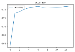
modeldf.loc[:, ['accuracy']].plot(title="accuracy")
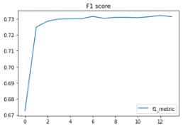
modeldf.loc[:, ['f1_metric']].plot(title="F1 score")
Our accuracy came in at 73% with an F1 score at .73 as well. Interestingly, the accuracy before we oversampled was 91%, but the F1 score was .08, which indicated the model wasn’t great (it was predicting everything as no). Oversampling clearly helped. Given the simplicity of the dataset, we found 73% accuracy to be impressive. Using more detailed data would have allowed us to produce a higher accuracy, but the more detailed data lacks the ability to easily be measured.